Mixed slabs¶

Homogeneous Mix of laboratory uniaxial materials at fixed volume fractions. Covers binary MixRule contrast and linear \(N\)-ary mixes.

Shared preamble:

from refloxide.model import MaterialSLD, FreeUniTensor, Mix, ReflectModel
from refloxide.profiles import (
    Diffusion,
    SecondOrderTransition,
    DepthProfile,
    Spline,
    Polynomial,
    CallableField,
    CallableDepthProfile,
)

vac = MaterialSLD("", 0, name="vacuum")(0, 0)
si = MaterialSLD("Si", 2.33, name="si")(0, 3.0)
mat = FreeUniTensor(energies=[284.4], name="film")
mat_a = FreeUniTensor(energies=[284.4], name="a")
mat_b = FreeUniTensor(energies=[284.4], name="b")
mat_c = FreeUniTensor(energies=[284.4], name="c")

Binary MixRule comparison¶

Builder: case_mixed_homogeneous

Every MixRule is a separate Mix instance at the same \(\phi\) (material A fraction \(0.3\)). Maxwell-Garnett takes host_index as the continuous phase (here material B):

phi_a, phi_b = 0.3, 0.7
materials = [mat_a, mat_b]
fractions = [phi_a, phi_b]

mixed_linear = Mix(materials, fractions=fractions, rule="linear")
mixed_mg = Mix(
    materials, fractions=fractions, rule="maxwell_garnett", host_index=1
)
mixed_bruggeman = Mix(materials, fractions=fractions, rule="bruggeman")

stacks = {
    "linear": vac | mixed_linear(200.0, 2.0) | si,
    "maxwell_garnett": vac | mixed_mg(200.0, 2.0) | si,
    "bruggeman": vac | mixed_bruggeman(200.0, 2.0) | si,
}

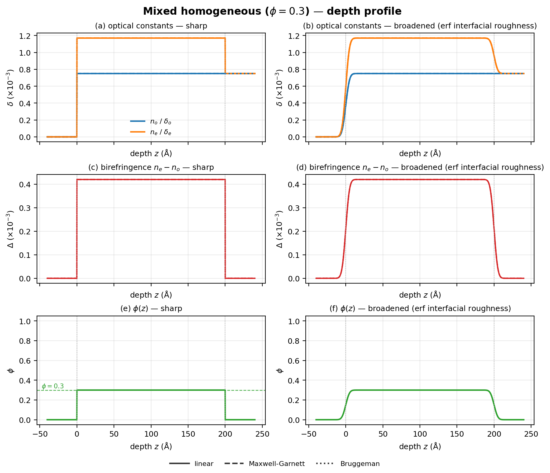
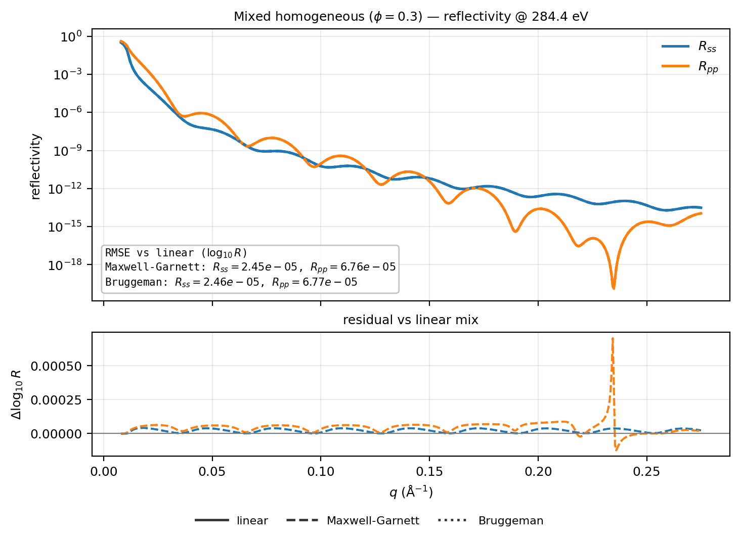
Fixed \(\phi=0.3\). Depth figure matches the CallableField template: left column sharp, right column erf-broadened; rows are optical constants (\(\delta\)), birefringence, and \(\phi(z)\). Channel keys use the common \(n_o/\delta_o\), \(n_e/\delta_e\) notation. Mix methods are linestyle only, with a bottom-centered legend (one column per method). Reflectivity keeps \(R_{ss}\)/\(R_{pp}\) color keys plus the same method legend; a residual panel and RMSE box show \(\Delta\log_{10} R\) vs the linear mix (soft-XR EMA curves nearly overlap on absolute \(R\)).

Mixing math¶

Channels are packed as \(\rho=\delta+i\beta\) with \(n=1-\delta+i\beta\) and \(\varepsilon=n^2\). Linear averages \(\rho\); Maxwell–Garnett and Bruggeman mix on \(\varepsilon\), then map back to \(\rho\).

Linear (volume-weighted channels; \(\phi\) = fraction of A):

\[ \rho_\mathrm{lin}=\phi\,\rho_A+(1-\phi)\,\rho_B \]

Maxwell–Garnett (host \(H\), inclusion \(I\), inclusion fraction \(\phi_I\); spherical EMA on \(\varepsilon\)):

\[ \alpha=\frac{\varepsilon_I-\varepsilon_H}{\varepsilon_I+2\varepsilon_H},\qquad \varepsilon_\mathrm{MG}=\varepsilon_H\frac{1+2\phi_I\alpha}{1-\phi_I\alpha} \]

Bruggeman (symmetric two-phase EMA on \(\varepsilon\); \(\phi\) = fraction of A):

\[ \phi\frac{\varepsilon_A-\varepsilon}{\varepsilon_A+2\varepsilon} +(1-\phi)\frac{\varepsilon_B-\varepsilon}{\varepsilon_B+2\varepsilon}=0 \]

Closed form with \(\gamma=(3\phi-1)\varepsilon_A+(2-3\phi)\varepsilon_B\):

\[ \varepsilon_\mathrm{Br}=\frac{1}{4}\Bigl(\gamma+\sqrt{\gamma^2+8\varepsilon_A\varepsilon_B}\Bigr) \]

After MG/Bruggeman, \(\rho\) is recovered from \(n=\sqrt{\varepsilon}\) (\(\operatorname{Re}n\ge 0\)) via \(\delta=1-\operatorname{Re}n\), \(\beta=\operatorname{Im}n\).

mixed homogeneous depth

mixed homogeneous reflectivity

\(N=1,2,3\) materials (linear)¶

Builder: case_mixed_homogeneous_nary

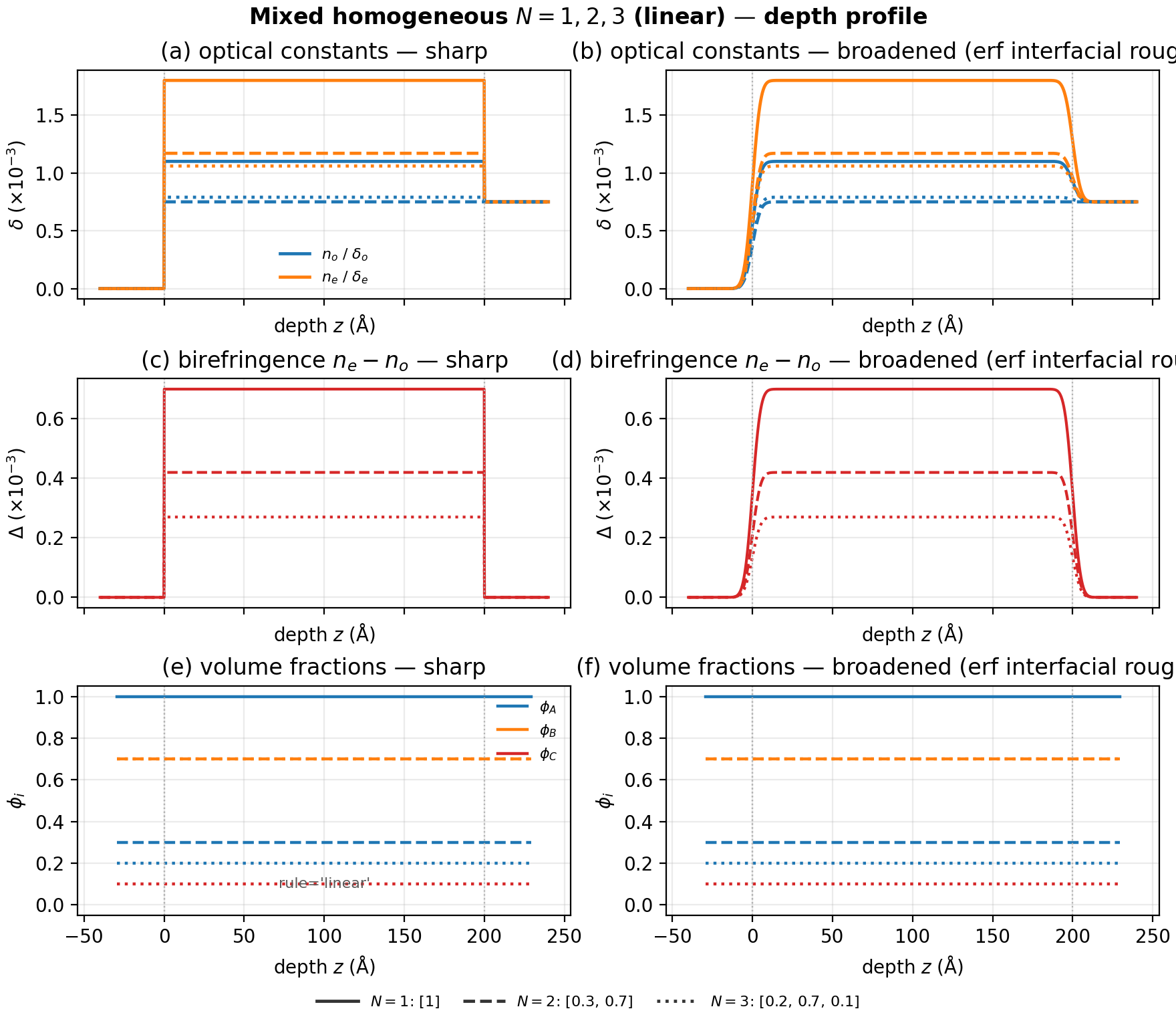
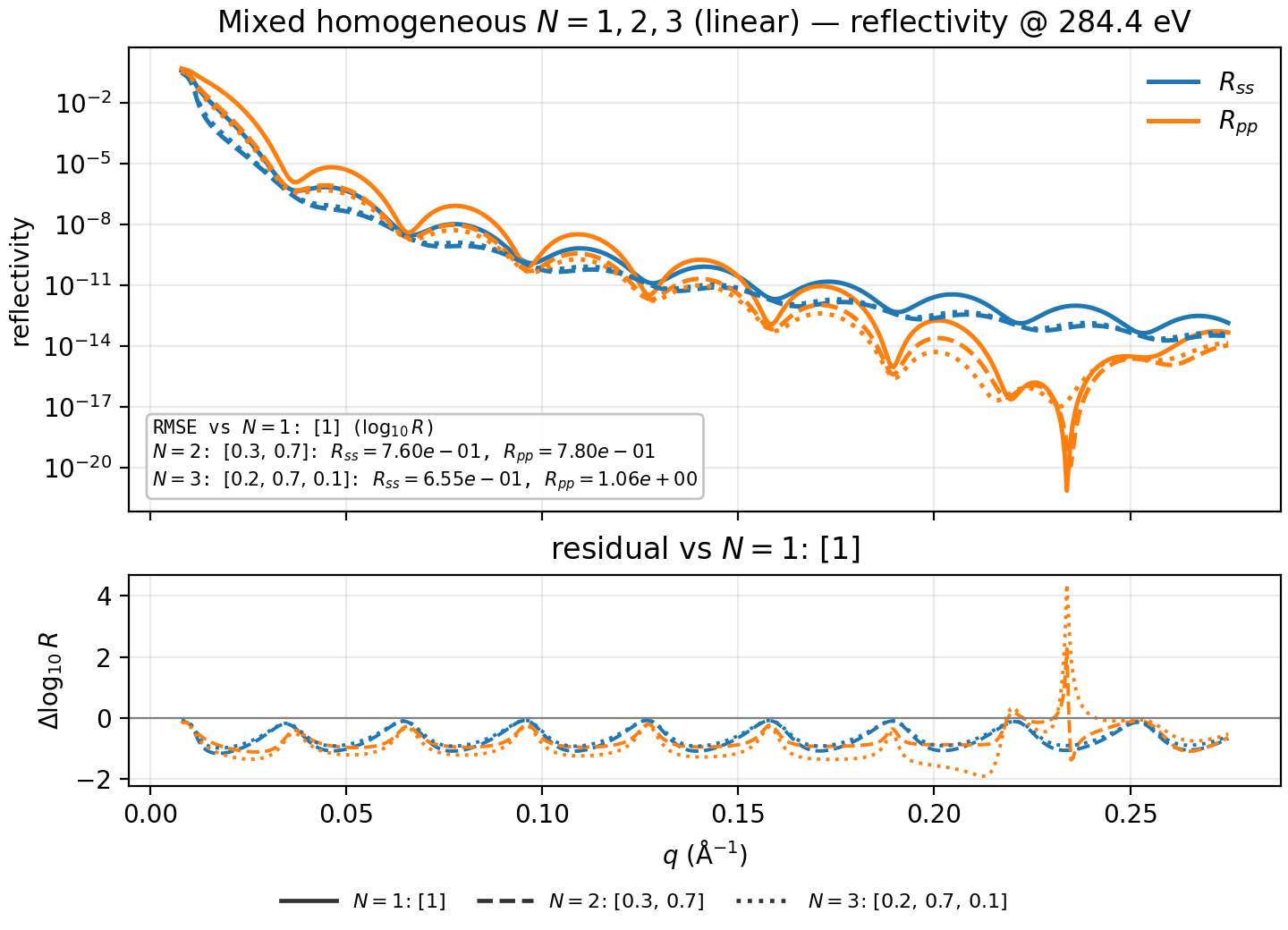
Same sharp | broadened depth template, but linestyle now marks the number of materials in a linear Mix (Maxwell–Garnett / Bruggeman remain binary-only). Fraction vectors are listed explicitly; reflectivity residuals are relative to the pure-\(A\) (\(N=1\)) slab.

mix_1 = Mix([mat_a], fractions=[1.0], rule="linear")
mix_2 = Mix([mat_a, mat_b], fractions=[0.3, 0.7], rule="linear")
mix_3 = Mix(
    [mat_a, mat_b, mat_c],
    fractions=[0.2, 0.7, 0.1],
    rule="linear",
)

stacks = {
    "N=1": vac | mix_1(200.0, 2.0) | si,
    "N=2": vac | mix_2(200.0, 2.0) | si,
    "N=3": vac | mix_3(200.0, 2.0) | si,
}

Bottom row of the depth figure draws horizontal lines at each listed \(\phi_A\), \(\phi_B\), \(\phi_C\) (color by material; linestyle by \(N\)).

mixed homogeneous n-ary depth

mixed homogeneous n-ary reflectivity

Stacking¶

A mixed film sits in a stack like any homogeneous slab:

mixed = Mix([mat_a, mat_b], fractions=[0.3, 0.7], rule="linear")
stack = vac | mixed(120.0, 2.0) | mat(80.0, 1.0) | si
model = ReflectModel(stack, energies=[284.4], parallel=False)