

ZnPc carbon K-edge NEXAFS
Zinc phthalocyanine (ZnPc) thin-film NEXAFS at the carbon K-edge, measured at five incidence angles (20°–90°). The goal: describe the spectrum as a sum of Gaussian peaks on a fixed continuum, then read off the matching \(\delta\) without any numerical KK transform.
Everything here runs from the data shipped in the package:
from lineshapes import datasets, mu_to_beta

t = datasets.load_table("znpc_nexafs")       # energy_ev, theta_deg, mu_cm2_per_g, intensity_raw
m = t["theta_deg"] == 54.7                   # magic angle: orientation-independent
E = t["energy_ev"][m]
beta = mu_to_beta(E, t["mu_cm2_per_g"][m])   # beta = mu * rho * lambda / (4 pi), per unit density
The script is examples/znpc_nexafs.py in the repository; make docs-figures regenerates the figures.
The recipe
- Start from the material's fixed continuum: bare-atom \(\beta\) (a line plus an erf ionization step at the C 1s ionization energy), with its \(\delta\) from kkcalc2.
- Add one Gaussian per seed. The seeds are DFT transition clusters: their energies and widths become the starting positions and widths.
- Solve the peak heights linearly (non-negative least squares) for the starting guess.
- Refine every peak's position, width and height, and the global density
scale, withscipy.optimize.least_squares, evaluating through a boundEvaluator.
def fit_peaks(energy, beta, material: str, seeds: dict, *, max_nfev=150) -> PeakFit:
    """Fit Gaussian peaks (plus the global scale) to ``beta`` on top of the fixed continuum."""
    e0s = np.asarray(seeds["energy_ev"])
    sigmas = np.asarray(seeds["sigma_ev"])
    widths = np.sqrt(2.0) * sigmas  # 1/e half-width of a Gaussian with std sigma

    cont = datasets.continuum_model(material)
    y = beta - cont(energy).imag  # what the peaks must explain
    basis = np.column_stack([Model().gaussian(e, w, 1.0)(energy).imag for e, w in zip(e0s, widths)])
    amp0, _ = nnls(basis, y)
    keep = amp0 > 1e-6 * amp0.max()  # a seed the data does not need stays out of the fit
    e0s, sigmas, widths, amp0 = e0s[keep], sigmas[keep], widths[keep], amp0[keep]

    model = datasets.continuum_model(material)
    for e, w, a in zip(e0s, widths, amp0):
        model.gaussian(float(e), float(w), float(a))
    seed_model = model.copy()

    names = model.param_names
    theta0 = model.params.copy()
    free = np.array([n.startswith("gaussian") or n == "scale" for n in names])
    lo, hi = np.full(theta0.size, -np.inf), np.full(theta0.size, np.inf)
    for i, n in enumerate(names):
        if n.endswith(".e0") and n.startswith("gaussian"):
            k = int(n.split("[")[1].split("]")[0])
            span = max(1.0, 1.5 * sigmas[k])
            lo[i], hi[i] = theta0[i] - span, theta0[i] + span
        elif n.endswith(".width"):
            lo[i], hi[i] = 0.1, 15.0
        elif n.endswith(".amp"):
            lo[i], hi[i] = 0.0, np.inf
        elif n == "scale":
            lo[i], hi[i] = 0.5, 1.5

    ev = model.bind(energy)
    buf = np.empty(energy.size, dtype=complex)
    norm = float(np.max(beta))
    theta = theta0.copy()

    def residual(p):
        theta[free] = p
        return (ev(theta, out=buf).imag - beta) / norm

    t0 = time.perf_counter()
    sol = least_squares(residual, theta0[free], bounds=(lo[free], hi[free]), x_scale="jac", max_nfev=max_nfev, ftol=1e-10, xtol=1e-10)
    seconds = time.perf_counter() - t0
    theta[free] = sol.x
    model.set_params(theta)
    r = model(energy).imag - beta
    return PeakFit(
        model=model, seed_model=seed_model, names=names, theta=theta.copy(), n_peaks=len(e0s), n_evals=sol.nfev,
        seconds=seconds, rms=float(np.sqrt(np.mean(r**2))), rel_rms=float(np.sqrt(np.mean(r**2)) / np.mean(beta)),
    )
Fit
The starting guess already captures the structure; refinement removes the remaining mismatch. The residual is at the level of the measurement noise, apart from a slow drift below the edge where the molecular spectrum departs from the bare-atom continuum.
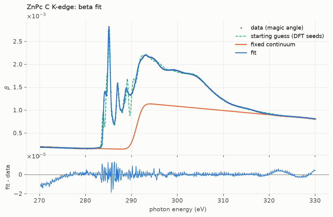
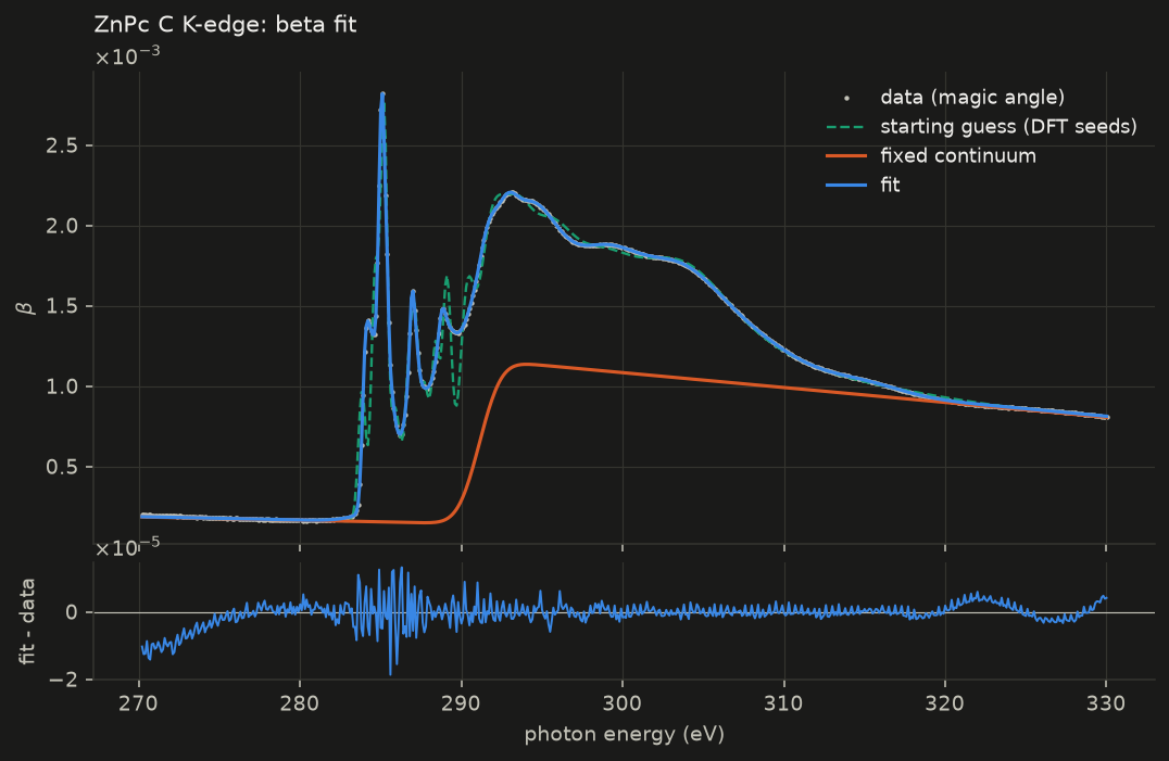
| # | E0 (eV) | 1/e half-width (eV) | height (beta) |
|---|---|---|---|
| 1 | 284.03 | 0.27 | 6.44e-04 |
| 2 | 284.40 | 0.41 | 8.93e-04 |
| 3 | 285.06 | 0.27 | 1.69e-03 |
| 4 | 285.28 | 0.61 | 8.67e-04 |
| 5 | 285.39 | 0.13 | 2.54e-04 |
| 6 | 286.75 | 2.64 | 1.77e-04 |
| 7 | 286.93 | 0.13 | 1.35e-04 |
| 8 | 286.99 | 0.32 | 5.39e-04 |
| 9 | 287.23 | 1.15 | 6.27e-04 |
| 10 | 288.79 | 0.30 | 1.85e-04 |
| 11 | 289.01 | 0.96 | 8.83e-04 |
| 12 | 290.43 | 1.03 | 7.17e-04 |
| 13 | 291.60 | 0.79 | 4.92e-04 |
| 14 | 292.69 | 0.87 | 2.91e-04 |
| 15 | 294.10 | 2.74 | 9.15e-04 |
| 16 | 298.68 | 3.03 | 5.74e-04 |
| 17 | 303.10 | 3.27 | 3.33e-04 |
| 18 | 305.63 | 5.74 | 3.81e-04 |
| 19 | 315.00 | 3.35 | 5.80e-05 |
Fitted density scale: 1.008 (the tables are per unit density).
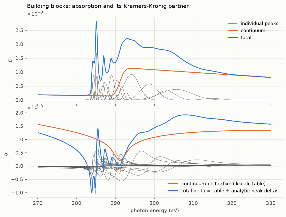
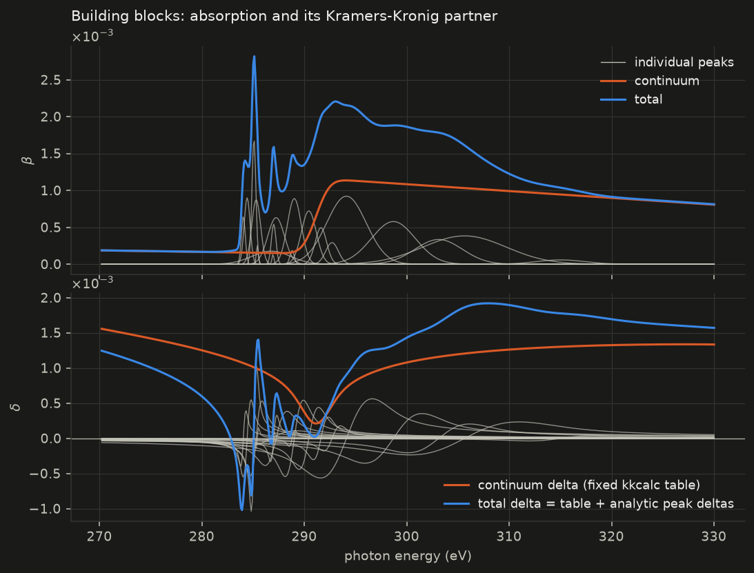
Absorption and its Kramers-Kronig partner
Each Gaussian contributes a bell in \(\beta\) and a dispersive Dawson-function shape in \(\delta\) (thin gray lines). The total \(\delta\) is the fixed continuum table plus the sum of the analytic peak partners: no transform was run to get it.
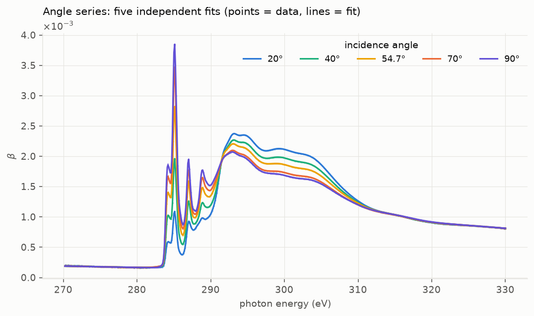
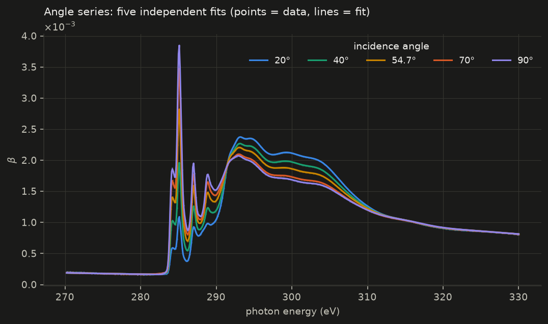
Five angles
The same recipe, applied independently to each incidence angle, with the same seeds. The strong angular dependence of the \(\pi^*\) resonances near 285 eV is the dichroism of the oriented molecular film. The library has no tensor machinery: each angle gives its own scalar optical constant, which is the building block for orientation-resolved models.
| angle | fit time (s) | model evaluations | rms residual / mean beta |
|---|---|---|---|
| 20° | 1.17 | 150 | 0.44% |
| 40° | 0.57 | 150 | 0.34% |
| 54.7° | 0.44 | 150 | 0.34% |
| 70° | 0.44 | 150 | 0.51% |
| 90° | 0.45 | 150 | 0.47% |
Fit times are for the machine that built these docs. Each fit refines 19 peaks (58 parameters including the scale) on 599 energies.